Get it
Python 3.10 or newer. Without numba the structures and the serial kernels still run, in pure Python; the threaded kernels need it.
git clone https://github.com/hellolulujiang/flowtopo.git
cd flowtopo
pip install -e .            # numpy + rasterio: structures and serial kernels
pip install -e ".[speed]"   # adds numba: the threaded kernels need it
Quick start
import flowtopo

topo = flowtopo.FlowTopo.from_raster("data/dir_example.tif")

upa = topo.upstream_area(ordering="dfs")           # km², one serial pass
ldn = topo.distance_to_outlet(ordering="dfs")      # flow length downstream, m
strord = topo.strahler_order(                      # on cells draining ≥ 10 km²
    ordering="dfs", channel_mask=topo.channel_mask(upa, 10.0))

upa_grid = topo.to_2d(upa)                         # back on the raster grid
Three of the kernels also run on threads, a layer at a time (needs numba); Strahler stream order runs serially only:
from flowtopo import parallel
upa = parallel.upstream_area(topo, layering="cfds", manner="push")   # push is safe only under cfds
Example data
data/dir_example.tif is the example basin of the paper: 292 rows by 614 columns at 3 arc-seconds, 93,432 valid cells, 731 km², cut from MERIT Hydro (Yamazaki et al., 2019) and kept under its CC BY-NC 4.0 terms. The GeoJSON files are the basin boundary and the outlet.
Any D8 GeoTIFF in the same convention works, as long as it is in longitude and latitude: the area and distance kernels treat the grid as degrees. Codes are powers of two clockwise from east; 0 and 255 are terminals; 247 is always nodata, and a nodata value declared in the file is excluded as well. Work one region or basin at a time: indices are int32, so a raster must stay under 2.1 billion cells, nodata included; the regions of MERIT-FullBasin do.
What you get
Eight structures, grouped by the question each one answers, and three ways to pass a value from a cell to its receiver. All are built from the D8 grid. Every clip runs on the same example basin; it plays while it is on screen, and opens full size on a click.
One core: in what order?
Three serial orderings. One pass over any of them computes a kernel. They differ in memory access, and so in speed.
ordering="topo"a cell is appended once all its donors are doneordering="bfs"cells in order of hop count from the pitordering="dfs"one tributary subtree at a time; best cache localityMany threads: which cells together?
Three parallel layerings. Layers run in order; the cells of one layer run at the same time.
layering="asap"every cell in the earliest layer its donors allowlayering="cfds"as soon as possible, plus: no two cells in a layer share a receiverlayering="alap"every cell as late as the longest flow path allows; the most evenly filled layers in practiceSeveral processors: which cells where?
Two spatial partitions, one subregion per processor. Both cut along the drainage hierarchy, so no value crosses a boundary while a kernel runs.
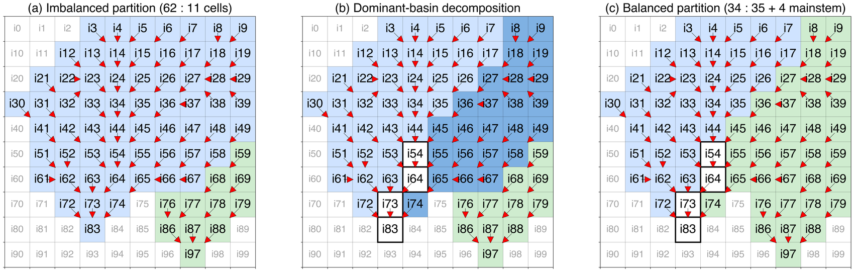
level="basin"Whole basins go to subregions; a dominant basin cannot be balanced.
level="subbasin"The dominant basin is cut along its mainstem; its tributary subtrees balance the load, and the mainstem runs in a separate stage.
At a confluence: how does a value reach the receiver?
Three propagation manners. The structure decides when a cell runs; the manner decides who writes the result.
manner="pull"each receiver reads its donors and writes only itself; needs the donor tablemanner="atomic_push"donors write through atomics; correct, but float sums are not reproduciblemanner="push"donors write directly; deterministic, no locks; safe only under cfdsThree things to know
- An ordering is built in one direction and can be read in either. Kernels that gather into the receiver (upstream drainage area, flow length upstream, Strahler stream order) walk upstream to downstream; flow length downstream walks the other way. The kernels pick the direction themselves;
topo.ordering("dfs", "u2d")asks for one explicitly. - The layer count is set by the longest flow path, and the conflict-free rule may add layers (on the example basin it adds none: 949 for all three). In the two headwater-anchored schemes layer 0 holds every headwater; in as-late-as-possible it holds only the farthest ones.
topo.partition(n_parts, level)returns a label per cell and the load per subregion. Subbasin-level marks the mainstemflowtopo.MAINSTEM; it runs as its own stage, after the tributary subregions for kernels that accumulate downstream and before them for flow length downstream.
Four kernels come with the package: upstream drainage area, flow length downstream (distance_to_outlet), flow length upstream (longest_upstream_path) and Strahler stream order. Each runs on every supported combination of structure and manner, and the results are checked against each other.
Write conflicts and cache locality on the example basin
A push is only safe if no two cells in a layer write to the same receiver. Conflicting writes inside a layer, example basin (93,432 cells):
| layering | conflicting writes |
|---|---|
| as-soon-as-possible | 12,122 |
| conflict-free downstream | 0 |
| as-late-as-possible | 39,130 |
The count is a property of the layering and can be checked before running. A test run cannot replace that check, because a race does not show up every time. Under the conflict-free layering no two cells in a layer share a receiver, so the push adds in the same order every time and gives bit-identical results at any thread count. Strahler stream order cannot be done with one atomic operation, because its confluence rule is a comparison and a count, not an addition; the only parallel push for it is under the conflict-free layering. When manner is not given, the FlowTopo methods pick a safe one for the layering; parallel.upstream_area defaults to push, which is safe only under cfds.
The three serial orderings differ in memory access. Simulated L1 miss rate on the example basin: depth-first 10.5%, breadth-first 21.8%, topological sort 37.1% (flowtopo.locality.miss_rates). The numbers move by a few points with how the two arrays sit in memory; the ranking does not.
Which structure to use
From the paper's benchmark of the C implementation on the 90 m network (22.2 billion cells, 65 regions):
- One pass on one core — the depth-first ordering. Up to 5.1 times faster than the slowest ordering, because each cell's receiver stays close in memory (L3 miss rate 6% against 37%). Measure parallel speedup against it; a slower baseline inflates the speedup.
- Repeated passes (calibration, ensembles) — the as-late-as-possible layering, fastest in parallel for all four kernels because each layer fits in cache. Under it, atomic push beat pull for sums and maxima (71.1 s against 85.1 s for flow length upstream). Use pull when the kernel has no atomic form or the result must be reproducible; pull needs the donor table.
- Push for a non-linear kernel, or little RAM — the conflict-free downstream layering with push. No locks, deterministic, only the receiver pointer stored, and the only push that can run Strahler stream order. Pull also runs it under any layering and was faster (4.8 s against 9.1 s); push wins when the donor table does not fit in memory.
- Across processors — the subbasin partition, one subregion per processor, with as many threads per subregion as the processor's memory bandwidth can feed. That number depends on the processor; measure it on yours.
The package runs numba over numpy on far smaller grids, and the ranking is not the same: on 16 million cells, push under cfds is the fastest threaded form and pull is slower than the serial pass, because building and reading the donor table costs more than ten threads save. Run benchmark.py on your machine before choosing; it times upstream drainage area on synthetic grids of the side length you give it.
Global products
Run with the C implementation over the 90 m MERIT Hydro network, the same methods produced two Zenodo records of per-region GeoTIFFs. Both cover the 65 continental regions of MERIT-FullBasin; the 29 island groups and the two regions that straddle the antimeridian are not included.
- MERIT-FlowTopo 10.5281/zenodo.20653059
- The structures: for every region the depth-first sequence, the conflict-free downstream and as-late-as-possible layerings and the subbasin partition; for Region 43 (southern China) all eight, so the alternatives can be compared in one region. 978 GB uncompressed, 50 GB compressed.
- MERIT-DrainAttr 10.5281/zenodo.20686665
- The kernels run over those structures: flow length downstream, flow length upstream and Strahler stream order for every region, and upstream drainage area for Region 43 only, since MERIT Hydro already distributes it globally. 622 GB uncompressed, 60 GB compressed.
- MERIT-FullBasin 10.5281/zenodo.20344113
- The companion dataset that divides the network into 96 hydrologically independent regions, the 65 continental ones being those above. On this site: FullBasin on MERIT Hydro · 90 m.
- MERIT-FlowTopo code 10.5281/zenodo.22227621
- The record the paper cites for code: the C implementation that produced the two records above, the scripts and data behind every figure, and an archived copy of the Python package (0.1.0).
Four maps over the 65 regions
Serial orderings: the sequence index of each ordering, globally and in the example basin
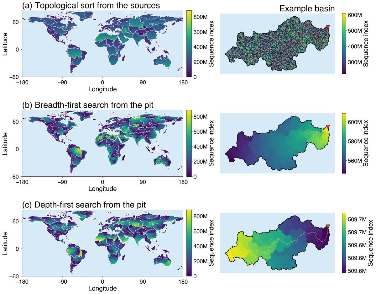
(a) topological sort from the sources, (b) breadth-first from the pit, (c) depth-first from the pit. The topological sort rises smoothly from headwaters to outlets, breadth-first forms bands of equal hop count from the outlet, depth-first breaks the basin into one compact block per tributary. Global maps share one scale from 0 to the total cell count; each basin map is scaled to itself; the red triangle is the outlet. All three are stored upstream to downstream.
Parallel layerings: the layer index of each layering; only as-late-as-possible fills its layers evenly
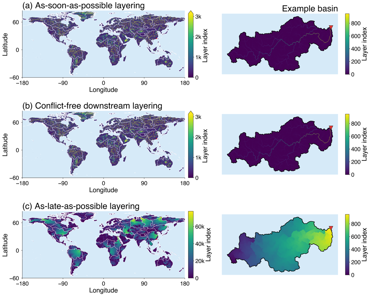
(a) as-soon-as-possible, (b) conflict-free downstream, (c) as-late-as-possible. Under (a) and (b) most cells sit in the first few layers and only the main rivers reach high indices, so the global scale is cut at 3,000; (c) spreads the cells over all layers and uses the full range, tens of thousands in the largest basins. The example basin has 949 layers under all three.
Spatial partitions: every region split four ways, Region 43 before and after the mainstem cut
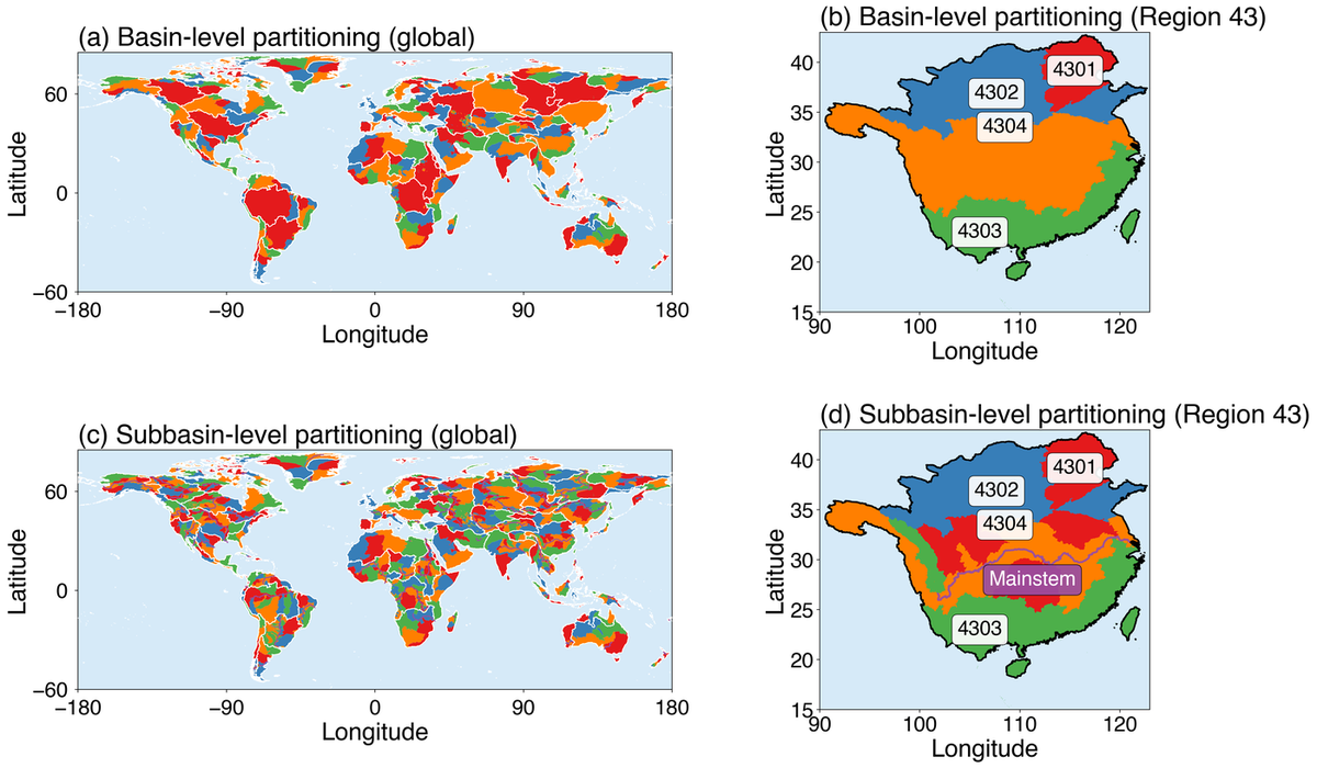
(a, c) all 65 regions; (b, d) Region 43, subregions 4301 to 4304. Top row basin-level: the dominant basin of Region 43 fills one subregion on its own. Bottom row subbasin-level: the basin is cut along its mainstem (purple) and the four subregions come out balanced. The four colours recur region by region.
Kernel products: the four MERIT-DrainAttr variables mapped
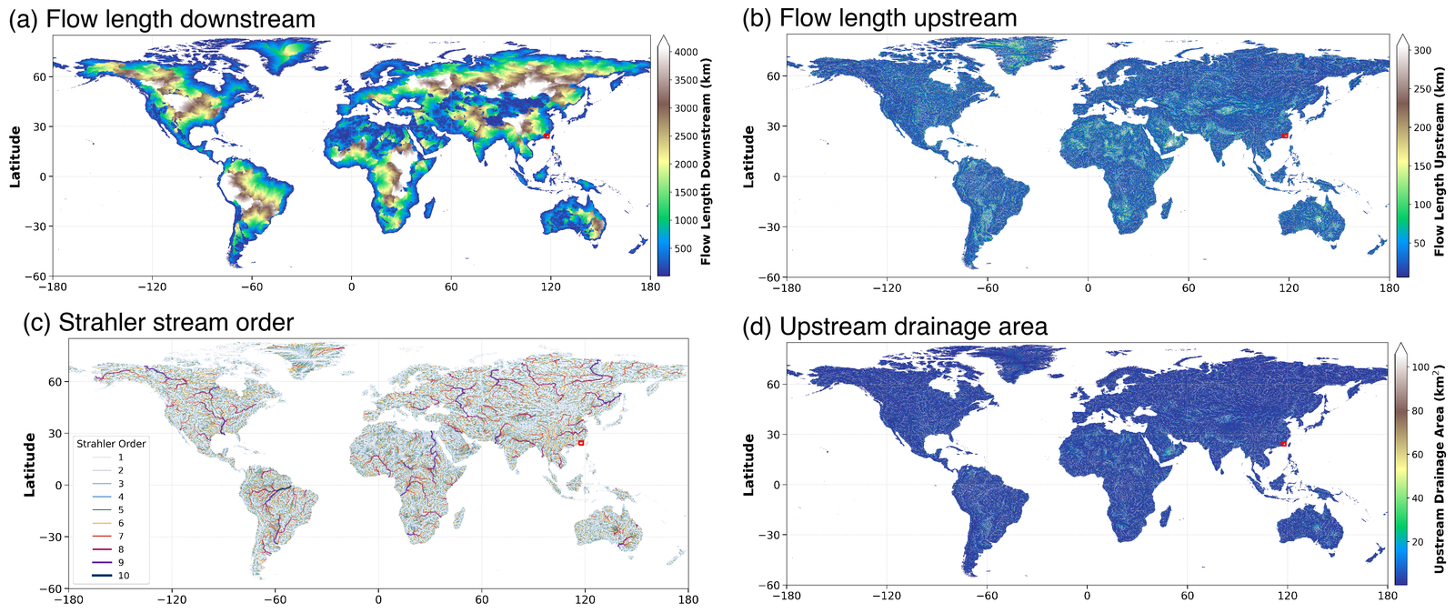
(a) flow length downstream, km; (b) flow length upstream, km; (c) Strahler stream order on channels draining at least 10 km²; (d) upstream drainage area, km², colour scale cut at 100 km². The red box is the example basin. (d) is released for Region 43 only, since MERIT Hydro distributes it globally.
Using the released structures
The structures index into the MERIT Hydro flow-direction grid, which is not redistributed: get it from the MERIT Hydro page under its own terms. Which MERIT Hydro tiles a region needs, and the row and column offset of each, is listed on the basin and region mask page of the 90 m collection. Region boxes sit on whole degrees and one degree is 1,200 cells, so a region is cut from the global rasters by integer arithmetic, with no resampling.
You do not need a whole region. Keep any subset of cells: the released sequence restricted to them is still a topological sort, and a restricted layering still has independent layers, conflict-free rule included, because removing cells cannot put a cell before something it depends on, nor make two remaining cells depend on each other. A receiver outside the clip becomes an outlet when the clip is loaded. Only the kernel values change: upstream drainage area on a clip counts the area inside the clip. Clip whole basins when the values must match the global ones, or take them from MERIT-DrainAttr.
The package is a port of the C code that produced the release. The two were written independently; on the example basin they agree to floating-point rounding in the accumulated area. That check has been made on the example basin only.
Documentation and checks
- User guide — choosing an ordering, a layering and a manner; threads; raster I/O.
- Methods — each method with its origin and its complexity, and what is borrowed from pyflwdir.
- Quick-start notebook — on the bundled data, stored with its output.
- Review checklist — what has been checked and how, the bugs those checks found, and what has not been checked yet.
pytest                  # needs pytest; numba for the threaded tests
python example.py       # every structure, kernel and manner on the example basin; ends PASS or FAIL
python benchmark.py     # serial vs threaded on synthetic grids
Every ordering, layering, partition, kernel and manner is cross-checked on the example basin, write-conflict counts included. The structures are checked against their definitions: an ordering is a topological sort, no cell in a layer depends on another cell of the same layer, and in an upstream-to-downstream sequence a receiver comes after its donors. All of that still holds after clipping a basin out of a region. The tests and example.py run on Python 3.10, 3.11 and 3.12 on every push.
Cite
The companion manuscript, MERIT-FlowTopo v1.0: a reusable computational foundation for hyperresolution hydrology on the global 90 m drainage network (Jiang et al.), was submitted to Geoscientific Model Development in September 2026; a citation will be added once it appears. Until then cite the code record 10.5281/zenodo.22227621, or the repository with the commit you used; for a downloaded product cite its version DOI above.
Acknowledgements
MERIT Hydro (Yamazaki et al., 2019) is the flow-direction grid everything here runs on. The flat downstream-pointer representation, the D8 decoding conventions, the donor-count array, the chain-tracing rank and the breadth-first sequence builder follow pyflwdir (D. Eilander, Deltares; MIT licence; 10.5281/zenodo.4287337). No pyflwdir source is included; the code was written against those conventions, and FlowTopo.from_d8 takes the same array pyflwdir.from_array(d8, ftype="d8") takes. Claude (Anthropic) assisted with the Python port, the tests, the documentation and the packaging; the authors reviewed the work, and the commit history records where. The methods and the results are the authors' own, described in the companion manuscript.
Licence
MIT for the code. The bundled MERIT Hydro excerpt keeps its own CC BY-NC 4.0 terms (DATA_NOTICE.md). Questions: [email protected], or a GitHub issue; email reaches us faster.
