Tested on
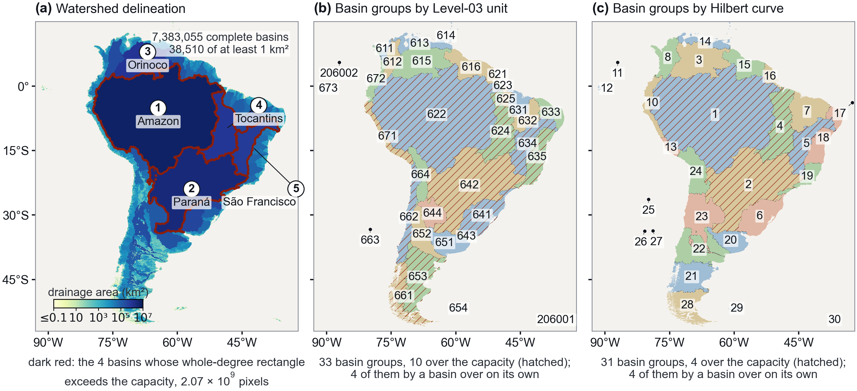
Tested on three large grids, all on one laptop with 64 GB of memory: HydroSHEDS v2 at 1 arc-second (30 m) over South America (259,200 × 219,600 pixels) and over North America (277,200 × 424,800), and MERIT Hydro at 3 arc-seconds (90 m) over the whole globe (174,000 × 432,000). On all three the results were compared with those of the C code.
How it works
Get it
Python 3.10 or later. A conda environment with GDAL is the easy way:
conda create -n flowdivide -c conda-forge python=3.11 numpy numba rasterio gdal pandas geopandas pyogrio pyarrow shapely scipy matplotlib
conda activate flowdivide
git clone https://github.com/hellolulujiang/flowdivide.git
The three grids above are built in; point the package at your downloaded copies with environment variables (see the user guide on GitHub), then
python flowdivide.py run south-america --out-root /data/flowdivide
python flowdivide.py run south-america --out-root /data/flowdivide --steps fd3 --capacity 2^31
Any other flow-direction grid, in any coding, projection or resolution:
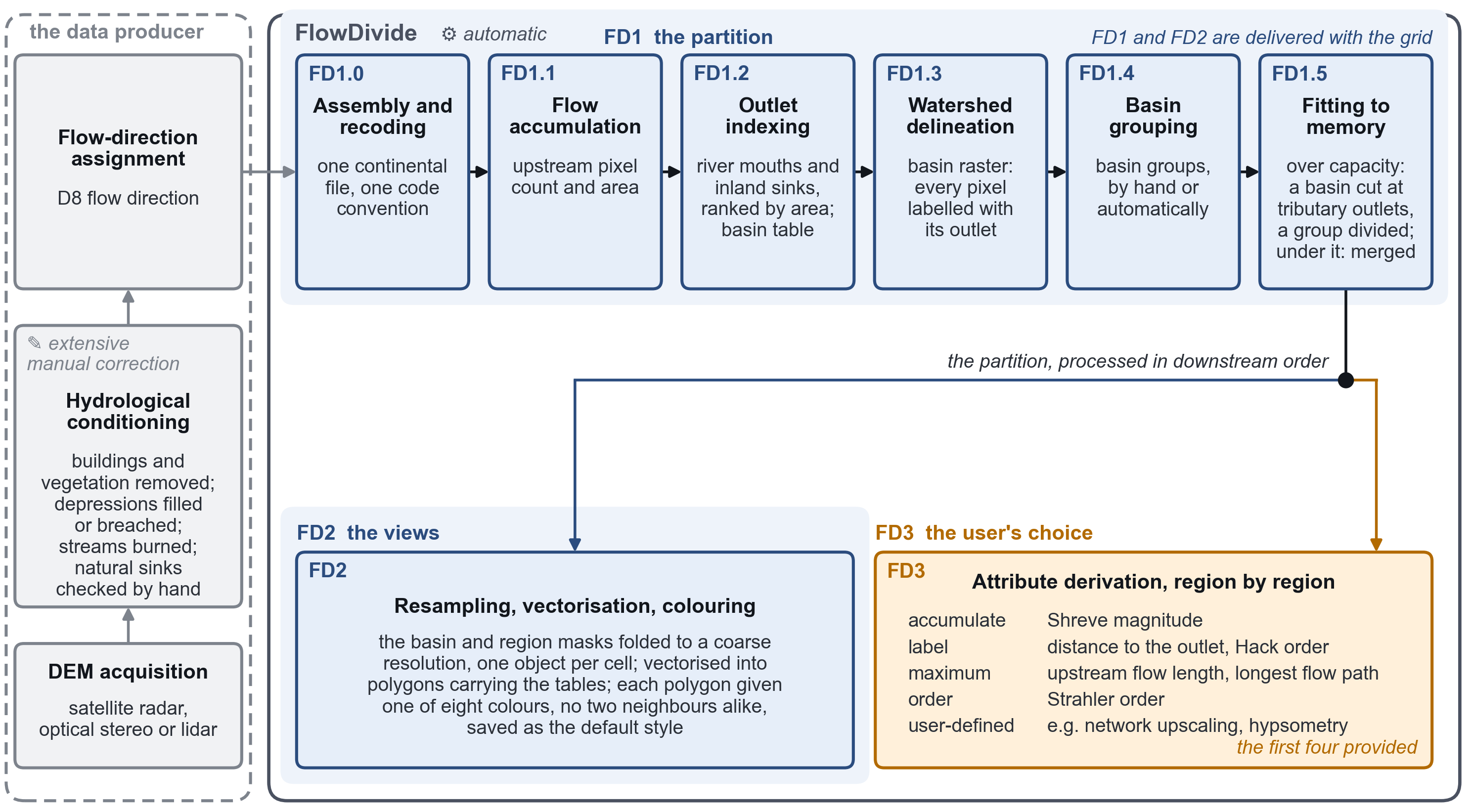
python flowdivide.py run mygrid --dir /data/mygrid_dir.tif --convention esri --out-root /data/flowdivideOut come the partition at three capacities (231, 230, 229 pixels), the basin and region tables, the coarse views as rasters and polygons (a GeoPackage opens in QGIS already coloured), and six attributes: Shreve magnitude, distance to the outlet, Hack order, upstream flow length, longest flow path and Strahler order. Every step checks its own output, and a stopped run resumes where it stopped.
Licence
MIT; see the licence. The grids FlowDivide runs on keep their producers' terms. Author: Lulu Jiang (lulujiang.me).
